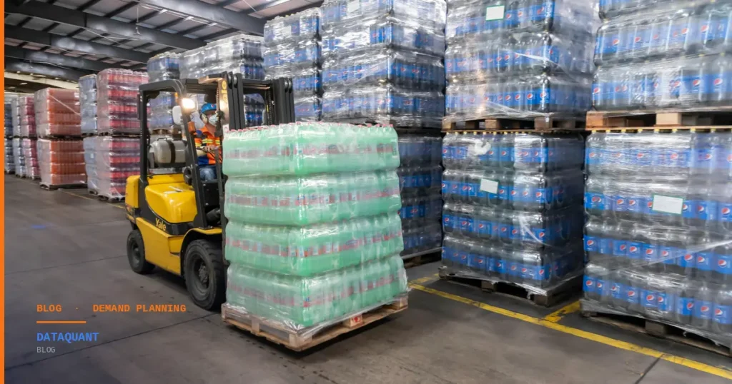
Demand Sensing for FMCG

From monthly forecast to daily signal in one quarter — a practitioner’s guide for Demand Planning Managers and Supply Chain Directors.

DATAQUANT RESEARCH TEAM  ·  DEMAND PLANNING  ·  11 MIN READ

The traditional FMCG demand planning cadence runs monthly. The S&OP cycle produces a forecast, the supply plan locks against it, and any deviation between the forecast and actual demand is reconciled the following month. This rhythm worked for decades when retailer order patterns were predictable, promotional calendars were locked in advance, and the cost of inventory imbalance was modest.

It works less well now. Retailer order velocity is faster. Promotional calendars are more dynamic. Direct-to-consumer channels generate signal at a daily — and sometimes hourly — cadence. Inventory imbalance is more expensive than it used to be, both in working capital and in stock-out cost as customers switch faster. The monthly cycle increasingly produces forecasts that are stale by week three of the month.

Demand sensing — the practice of incorporating short-cycle signals (1–7 day) into the demand forecast to update it continuously — has been talked about in FMCG for fifteen years. It has been fully implemented at a small minority of large CPG brands. The reason most FMCG businesses haven’t deployed it is not that the technology is unavailable; it is that the data architecture, model design, and process integration are non-trivial, and most planning teams have not had the analytical resources to bridge the gap.

This piece walks through what demand sensing actually is in practical terms, what data and models it requires, and what an FMCG demand planning team can realistically achieve in one quarter — starting from a typical monthly-cycle baseline.

What demand sensing actually is

Demand sensing is not a single technique. It is a layered approach that combines three forecasting horizons:

• Strategic forecast (12+ months): long-cycle drivers — macroeconomic, demographic, category trend, brand position. Updated quarterly. Used for capacity planning, supplier contracts, and budgeting.
• Operational forecast (1–12 weeks): medium-cycle drivers — promotional calendar, distribution changes, seasonality, weather, holiday calendar. Updated weekly. Used for production scheduling and replenishment.
• Sensing layer (1–7 days): short-cycle drivers — retailer POS, weather actuals, social/search signal, competitor price moves, supply-chain disruption signals. Updated daily. Used for production rate adjustments, inventory rebalancing, and pre-emptive stock-out prevention.

A working demand sensing capability does all three layers, with each layer informing the next. The sensing layer is the new piece for most FMCG businesses; the strategic and operational layers are usually already in place.

What signal the sensing layer actually picks up

The signals that drive demand sensing in FMCG cluster into four categories:

Signal 1: Retailer POS at sub-weekly granularity

The single most-valuable sensing input is daily retailer POS data — not weekly aggregates, not monthly summaries. Daily POS reveals: a SKU that is starting to accelerate ahead of plan, a SKU that is trending below plan despite a stable promo, a region where local conditions are pulling demand differently from the national pattern. The information arrives 2–7 days before the operational forecast would surface the same signal.

Retailer data-sharing varies materially across retailers. Some share daily SKU-level POS readily; some share only weekly category aggregates. The sensing capability is bounded by the quality of retailer data feeds, and improving those feeds is part of the work.

Signal 2: Weather actuals and short-range forecast

For weather-sensitive categories — ice cream, soft drinks, beer, soup, hot beverages, sun care, fresh produce — weather signal is the largest short-cycle driver of demand variance. Daily weather actuals (temperature, precipitation, humidity) plus 7-day forecasts feed into the sensing model and update the demand projection.

A typical pattern: a hot week produces 20–40% lift in beer and soft drinks at a regional level. The operational forecast does not capture this until the weekly POS comes in three days late. The sensing layer captures it in real time and adjusts production and replenishment within 24 hours.

Signal 3: Social and search signal

For brands with strong consumer engagement, social media velocity and Google Trends data correlate (with lags of 1–10 days, depending on the category) with subsequent demand. The signal is noisier than POS or weather but adds incremental information for products where consumer enthusiasm shifts quickly.

In our experience this signal is most useful for: snack/confectionery launches, seasonal items, products affected by viral content (a recipe, a celebrity mention, a TikTok trend), and limited-edition releases. For staple categories with stable consumption, search/social adds little.

Signal 4: Supply-chain and competitor disruption

When a competitor product goes out of stock at a major retailer, demand for substitute products in the same category accelerates within 24 hours. Demand sensing models that incorporate competitor stock-out signal (often available through retailer data feeds or third-party stock-tracking services) can pre-emptively adjust replenishment to capture the share gain. Conversely, when your own supply chain is disrupted, sensing-layer demand projections can be reset against revised supply availability rather than maintaining a forecast that would now produce stock-outs anyway.

A practitioner’s recipe for one quarter

For a demand planning team starting from a monthly cycle and wanting to deploy a working sensing layer in 12 weeks, the recipe looks like:

Weeks 1–3: Data architecture

Pipe daily retailer POS into a central warehouse table. For most FMCG businesses this requires negotiation or contract amendment with 2–3 major retailers; the rest can be approximated through panel data (Nielsen, IRI). Add weather feeds (Open-Meteo, Tomorrow.io, or local meteorological services). Add Google Trends for a curated set of category and brand keywords. The output of this phase is a unified daily-cadence dataset covering the past 24–36 months.

Weeks 4–7: Sensing model build

Build a model that takes the operational forecast as a baseline and produces a daily-update adjustment. The model architecture matters less than the data: gradient-boosted regressors (LightGBM, XGBoost) work well for this; some teams prefer hierarchical Bayesian models for the uncertainty quantification. Train on the past 18–24 months; validate on the most recent 6 months held out.

Performance target: at a 7-day forecast horizon, the sensing-adjusted forecast should improve MAPE by at least 10–15% versus the operational forecast alone, on validation data. If it does not, the data layer is the issue, not the model.

Weeks 8–10: Process integration

The sensing-layer output must feed into operating decisions. Three integration points:

• Production scheduling: daily production-rate adjustments based on the sensing-layer demand projection vs locked production schedule
• Replenishment: SKU-region replenishment rebalancing using daily sensing output, refreshed nightly
• Stock-out alerting: pre-emptive flags 3–5 days before a SKU-region combination is forecast to stock out

Weeks 11–12: Outcome measurement

Establish the measurement that proves the capability is producing value. Three KPIs are usually sufficient: forecast MAPE at 7-day horizon, stock-out rate by SKU-region, working-capital tied up in inventory. All three should improve in the first quarter of operation.

What this looks like in practice

A €420M confectionery manufacturer we worked with deployed a sensing layer over a 13-week engagement. Their operational forecast was running at MAPE 22% at 7-day horizon — the planning team had been frustrated for years. Stock-outs ran at 4.1% of SKU-region-week combinations. Working capital tied up in finished-goods inventory was 47 days.

After the sensing layer went live: 7-day MAPE fell to 17% within the first month, and to 14% within three months as the model accumulated more recent data. Stock-out rate fell to 2.6%. Inventory days came down to 39 — releasing approximately €11M of working capital. The capability paid for itself within four months on inventory release alone, before counting the recovered margin from reduced stock-outs.

Three pitfalls

1. Trying to replace the operational forecast rather than augment it. The sensing layer is an adjustment to the operational forecast, not a substitute. Teams that try to start from scratch with sensing produce models that handle short-cycle signal well and long-cycle drivers poorly. The hierarchical structure — strategic + operational + sensing — is what works.
2. Underestimating the weather model. For weather-sensitive categories, weather can be 30–60% of short-cycle demand variance. Treating weather as a generic input rather than a primary driver produces models that miss the largest signal in the system. Spend disproportionate effort on weather-feature engineering.
3. Building the model before negotiating retailer data feeds. A sensing model built on weekly POS data will be measurably less accurate than one built on daily POS. The retailer-data conversation is part of the project, not a precondition. Most major retailers will provide daily SKU-level data to suppliers who ask formally and have a credible analytical use case.

Closing thought

Demand sensing is not a destination — it is a layered capability that gets better as the data layer matures. The 12-week target outlined here produces a working sensing layer with measurable accuracy improvement and operational integration. The next iteration adds more signals, more retailers, finer SKU granularity. The destination is a planning function that operates at the cadence the market actually moves at — daily, with weekly review — rather than the monthly cadence that worked when the world was slower.